MATHEMATICA CAS IN PROCESSING AND INTERPRETATION OF GRAVITY AND MAGNETIC ANOMALIES

TÔN TÍCH ÁI

Department of Physics, University of Natural Sciences, VNU, Hà Nội

Abstract: The article contains different techniques of geophysical data processing and interpretation. Numerical methods are used for calculating gravity normal values according to the latitude. The paper also concerns with the calculation of gravity effect of different geological bodies with arbitrary shape. Equalization of basic gravity network is included for its use in practice with complex gravity basic network. Interpolation of simulation data is considered for calculation of different derivatives, used in the interpretation of received geophysical data. Transformation theory of geophysical data in frequency domain, presented in the paper finds good application for geophysicists, interested in geologo-geophysical interpretation of data. The calculation process is realized by using the Mathematica Computer Algebraic System (Mathematica CAS).

I. INTRODUCTION

The numerical simulation of various natural and technological processes or phenomena with the aid of computers has been now becoming a powerful tool for studying these processes or phenomena. In this paper, the numerical computation and computer graphics for purpose of processing and interpretation of potential geophysical data are used intensively. The needed numerical and symbolic computations are performed in our paper with the aid of the advanced Mathematica Computer Algebraic System (CAS). We show in our paper how this system can be used. The development of program package Mathematica was initiated by Stephen Wolfram in the 1980s. Now versions of Mathematica are available for wide variety of computer system. Mathematica Version 6 was first released in 2008. We will describe in our paper the application of Mathematica for processing and interpretation of potential field methods in geophysics. This article discusses these two uses.

II. PROCESSING OF GRAVITY DATA

In this part of the paper we will deal with some problems of calculating gravity normal values at different latitudes, adjusting basic gravity network and interpolating measured geophysical data.

1. Fast calculation of normal gravity values at different latitudes

We use the international formula for computing the normal sea-level gravity at latitude (GRS-1967). The formula is [3]

Gal (1)

Using Mathematica the function is defined as follows:

g [phi]:=978.0318(1+0.0053024sin [phi degree]^2-0.00000sin[2phi degree]^2).

From this formula, we may easily calculate the normal gravity values for different latitudes without regarding standard table:

Table [{phi,g[phi]},{phi,1,25,.5}]//InputForm

{{1, 978.0333795598982}, {2, 978.0381163151427}, {3, 978.0460044947265},

{4, 978.0570344881181}, {5, 978.0711928569697}, {6, 978.0884623514894},

{7, 978.1088219314587}, {8, 978.1322467918656}, {9, 978.1587083931254},

{10, 978.1881744958536}, {11, 978.2206092001427}, {12, 978.255972989302},

{13, 978.2942227780015}, {14, 978.3353119647657}, {15, 978.3791904887497},

{16, 978.4258048907312}, {17, 978.4750983782416}, {18, 978.5270108947595},

{19, 978.5814791928802}, {20, 978.6384369113727}, {21, 978.6978146560302},

{22, 978.7595400842176}, {23, 978.8235379930088}, {24, 978.8897304108098},

{25, 978.9580366923559}}.

2. Equalization of basic gravity network

The field routine for gravity measurements is similar to that for an elevation survey. Gravity differences are determined for a network of basic stations with respect to a starting point (base station) after allowing for drift. Closure errors for the network are eliminated by different methods of equalization. In this article the polygon method is considered.

We consider the network at the Fig. 1, in which the gravity differences are included near the sides of the polygons, the arrows indicate increase directions of , p_i is quality weights of measurements, v_i - closure errors.

Figure 1. Basic gravity network

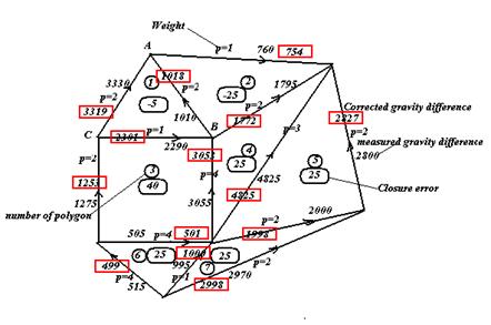
Calling k_i being correction values for weight unit of each polygon, according to [7], we have following equations for calculation of k_i:

eq1 =

eq2 =

eq3 =

eq4 =

eq5 =

eq6 =

eq7 =

(2)

Solving these equations with the aid of Mathematica (Solve[{eq1,eq2,eq3,eq4,eq5,eq6,eq7},{k₁,k₂,k₃,k₄,k₅,k_6,k₇}]) we receive the k_i values: k₁=-21.5858, k₂=-6.06507, k₃=-45.1391, k₄=-52.6745, k₅=-53.2402, k₆=-56.8574, k₇=-62.0948.

Now, we calculate the corrected gravity differences for all sides of network. We consider two cases: single side and common side between two polygons. For example, we calculate:

By similar method, we calculate all corrected gravity differences for all sides of the network.

3. Interpolation, approximation and their applications

Suppose is a set of geophysical data where x₀< x₁<… <x_N. We do not have an analytic expression of a function f whose graph contains these points, yet we want to calculate its value at an arbitrary point. For this purpose, we find the polynomial P_N(x) of degree not higher than N, whose values at point x_i coincide with the values of data, i.e. P_n(x_i)=y_i [6]. In this paper, we use Lagrange’s and Spline interpolations. Lagrange’s polynomial interpolation has the following form [6]:

(3)

where (4)

Spline interpolation uses polynomial n degrees in intervals (x_j, x_j+1) and using different conditions for calculating different coefficients in the polynomial.

In Mathematica, there are 2 commands for using interpolation: Interpolating-Polynomial [data, {vars}]; Interpolation [data].

The following table for the simulation of gravity anomalies is given:

x	(mGal)	x	(mGal)
-1000 -900 -800 -700 -600 -500 -400 -300 -200 -100	0.0284305 0.0329207 0.0385575 0.0457655 0.0551856 0.0678237 0.0853379 0.110644 0.149361 0.213976 0.338755	100 200 300 400 500 600 700 800 900 1000	0.612007 0.779651 0.826098 0.884819 0.748206 0.527098 0.354403 0.243304 0.17357 0.128626

With these data, Spline interpolation is applied for receiving function and is calculated. Received results indicate the ability of using interpolation approach in processing geophysical data.

III. MATHEMATICA CAS IN THE COMPUTATION OF GRAVITY ANOMALIES

Mathematica CAS may be used in two ways in the computation of gravity anomalies. The first way involves its use for contouring charts or templates which can then be manually used for computation of anomalies. The second is for direct application in the computation of the gravity and magnetic effect of bodies of arbitrary shape by developing the expressions for attraction as recursive formulas that are conveniently handled by computer.

1. Horizontal cylinder, horizontal line element

We choose the coordinate system of Fig. 3 such that the horizontal cylinder is parallel to the y axis and has the parameters h and R.

In this system we have [7]:

(5)

For calculating the gravity effect of horizontal cylinder, in Mathematica we may use the following commands:

Clear ["Global`*"]; sl = {k->66.73 10^-7, sig->500; h->200, R->100, x0->150};

f[x_] = 2k Pi R^2 sig h/((x-x0)^2+h^2); Plot [f[x]/.sl, {x, -700, 700}].

2. Horizontal rectangular parallelepiped

Gravity effect of rectangular parallelepiped is determined by following formula:

(6)

Results of calculation by Mathematica for 2 horizontal rectangular parallelepipeds are presented in Fig. 4:

Clear["Global`*"]; SetOptions[Plot, PlotStyle->Thick];

sl1 = {k->66.73 10^-7, sig->100., x1->250., x2->400., z1->50., z2->350.};

sl2 = {k->66.73 10^-7, sig->500., x1->750., x2->1500., z1->450., z2->750};

f[xi_, x_, z_] = k sig((x-xi)log[(x-xi)^2+z^2]+2z ArcTan[(x-xi)/z]);

f1[xi_, x_] = f[xi, x, z2]-f[xi, x, z1];

f2[xi_]=f1[xi, x2]-f1[xi, x1];

p1 = Plot [(f2[xi]/.sl1)+(f2[xi]/.sl2),{xi, -500, 2000}].

With the similar way we may calculate the gravity effect of different shapes of geological bodies.

IV. TRANSFORMATION OF GEOPHYSICAL DATA

The main purpose of separation (transformation) of potential (gravity and magnetic) fields is the extraction from observed field into components that are associated with individual geological objects located at different depths. The resulting function, depending on transformed operations may be of the same unit of initial function or their derivatives. Derivatives of initial function may be taken at started level or at new ones. The transformed function may have unit of product of initial function and coordinates.

Before eighty years, due to low technique and poor computing tool, most problems of field transformation were mainly carried out in space domain. At present, these problems, in general tendency, will be implemented in frequency domain with assistance of Fast Fourier or of other software.

Transformation in Space Domain

The mathematical expression of popular field transformation in space domain can be drawn out [5]:

- Averaging: The average of observed field is taken within the circle of radius R at the centre of circle:

(7)

- Analytical continuation of the field from 0-level to Z-level is expressed by:

(8)

- Derivatives undertaken along x-axis can be written:

(9)

- Derivatives calculated with respect to z-axis:

(10)

In particular way, for calculating above-mentioned transformations, the palettes designed for that purpose are used. Furthermore, these analytical expressions are suitable for computer calculations.

Transformation is carried out in frequency domain

In this domain all above-mentioned transformations can be expressed in common formulae:

- For 3D problems:

(11)

- For 2D cases:

(12)

where: ,,, are initial fields; , - transformation kernels corresponding respectively to 3D or 2D problems.

Expressions (11) and (12), which are integrals of 2 functions, are called as convolution. Mathematically, the process of signal filtering is described by such integrals. That is the problems of potential field transformation that can be considered as frequency filtering, in which various transformation operations are realized with different frequency characteristics.

According to the theory of convolution in the frequency domain, spectrum of function or is the multiplication of ones of and , i.e.

(13)

(14)

where the spectrum of functions is , is spectrum (frequency characteristics) of function .

Using direct Fourier transform, in formula (13) is calculated and after that, by inverse Fourier transforms, function is determined. Table 1 gives the frequency characteristics for different transformations of potential data.

Table 1. Transformation and its frequency characteristics

Transformation	Frequency characteristics
- Average: · 3D Problem · 2D Problem
- Analytical Continuation · Upward continuation · Downward continuation
- Vertical derivatives of n-order · On the observed surface · At the height z
- Horizontal derivatives of n- order · On the observed surface · At the height z

Transformation methods in frequency domain are realized on received geophysical data with accepted results.

V. CONCLUSIONS

We have used Mathematica CAS for processing, calculation and enhancement of geophysical data for determining their cause. Simulation results give us the opportunities of their use in practice.

REFERENCES

1. Bahder T.B., 1995. Mathematica for scientists and engineers. Addison-Wesley Publ. Co.

2. Nikitin A.A., 1993. Statistical processing of geophysical data. Electromagnetic Res. Center, Moscow.

3. Sharma P.V., 1997. Environmental and enginneering geophysics. Cambridge Univ. Press.

4. Tafeev G.P, Sokolov K.P., 1981. Geological interpretation of magnetic anomalies. Nedra, Leningrad.

5. Tôn Tích Ái, 1988. Applied geophysics. Univ. Min. Publ., Hà Nội.

6. Tôn Tích Ái, 2000. Computational method. Nat. Univ. Publ., Hà Nội.

7. Tôn Tích Ái, 2003. Gravity and gravity prospecting. Nat. Univ. Publ., Hà Nội.

8. Tôn Tích Ái, 2005. Geomagnetism and magnetic prospecting. Nat. Univ. Publ., Hà Nội.

9. Wolfram S., 1988. Mathematica. Addison-Wesley Publ. Co.