INTERPRETATION OF SOUNDING CURVES IN HỒ CHÍ MINH CITY BY ZOHDY METHOD

¹NGUYỄN THÀNH VẤN, ²LÊ NGỌC THANH, ³NGUYỄN NGỌC THU,
¹NGUYỄN THỊ NHƯ VƯƠNG, ¹NGUYỄN NHẬT KIM NGÂN

¹University of Natural Sciences, VNU-HC;
²Hồ Chí Minh City Institute of Geographic Resources, VAST ;
³Geological Mapping Division of South Việt Nam.

Abstract: Resistivity, one of physical parameters of material, plays an important role in many fields of research and application. Especially in geotechnical field, it is a necessary parameter to estimate the effect in underground construction, to protect the buildings from electrochemical effects and designing lightning-conductors, etc.

Some methods can be used to get the true resistivity of geological environment, in which vertical electric sounding (VES) is one of the most usual methods, that has been used for the resistivity testing.

In this paper, we introduce the average resistivity maps of Hồ Chí Minh city, based on the Zohdy method, the traditional and Dudás formulas with a huge of VES points.

I. AUTOMATIC INTERPRETATION OF RESISTIVITY SOUNDING CURVES BY ZOHDY METHOD

1. Theory of the method

Using the basic problem in resistivity sounding measurements based on a horizontally layered model, the potential U(r) at the surface of the layered earth is:

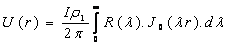(1)

where: J₀(lr) - Bessel function; R(l) - the kernel function.

With symmetric four-electrode configuration, the potential difference between the measuring electrodes is:

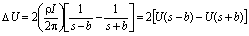(2)

where

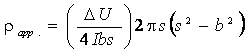
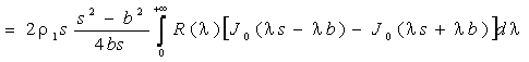
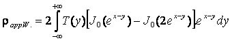
Thus, the expression for the apparent resistivity equation is:

(3)

or (4)

where T(l) = r.R(l) , c = b/s.

· In a special case for the Wenner electrode configuration, we have 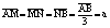(a - the distance between consecutive electrodes) and . Substituting these values into eq. (4), we obtain:

(5)

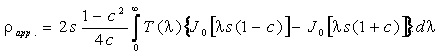
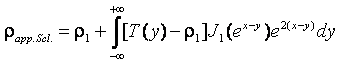
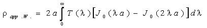
· With the Schlumberger electrode configuration, the formula of apparent resistivity is obtained in the form

(6)

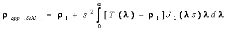
We replace the independent variables by logarithmic ones. The advantage of logarithmic variables over a linear scale for the independent ones is that the curves have the more regular appearance on the logarithmic scale.

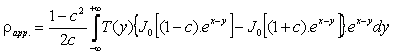
The variables x and y that are defined as x = ln(s), y = ln(1/l) = -ln(l). With the above changes, eqs. (4), (5) and (6) become

According to the Fourier transform, if a function T(y) is sampled at sample distances (y₀ + jDy) then the value of the function at an abscissa value y would be obtained as:

From this

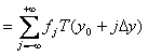
where f_j - filter coefficients.

Setting h = x - y, the filter coefficients may be written as:

Now, there are many filters with different sampling intervals (6, 10, 11,…) per decade. For example, Johansen’s filter and Ghosh’s filter with 140 and 9 corresponding filter coefficients are used. Here we choose Abramova’s filter with 15 filter coefficients.

The purpose of digitizing the sounding curves is to speed up the computations of the succession of theoretical sounding curves used in the iterative process.

2. Interpretation of the Zohdy method

On the basis of the above mentioned theory, the automatic interpretation of sounding curves is carried out by the following steps:

a. Plotting observed curve on a logarithmic scale (including electrode spacing (AB/2) and apparent resistivities scales) from field data points.

b. If electrode spacing (AB/2) have N values, the interpretation will automatically determine that the model has N layers. The j^th layer thickness is AB_j/2 – AB_j-1/2; the j^th layer resistivity r_j is also j^th layer apparent resistivity r_app.j. A number of layers does not change throughout the interpretation (Fig. 1a).

c. Based on the above assumed model with the parameters determined from step b, the program will solve forward problem with Abramova’s filter having 15 filter coefficients; plotting the calculated curve (Fig. 1b), then computing root-mean-

square (rms) percent from the equation:

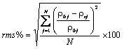
where: r_0j - j th “observed” apparent resistivity; r_cj - j^th “calculated” apparent resistivity; N - number of digitized apparent resistivity points (with j = 1 to N).

We compare the rms percent with the given condition. If the rms percent is minimum (less than 5 percent or a prescribed limit), the iterative process will be terminated. Then, the assumed depths and resistivities are also the true ones. If the above condition is not satisfied, we reach the next step.

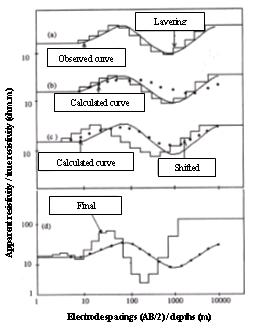
Figure 1. Basic steps in the qutomatic irritation method

d. Change in the layer depths and resistivities (Fig. 1c).

The depths decrease for each iteration. For the stability all the layer depths are reduced by 10 percent. The amplitude of a layer resistivity is iteratively adjusted as:

where i - number of iteration; j - j^th layer and spacing; r_i(j) - j^th layer resistivity at the j^th iteration; r_ci(j) - calculated apparent resistivity at the j^th spacing for th j^th iteration; r₀(j) - observed apparent resistivity at the j^th spacing.

With the new values, in repeated step b) the assumed depths and resistivities are equal to the adjusted ones. The iterative process is continued until the condition of step c) is met (Fig. 1d).

3. Method for the calculation of average resistivity

After calculating the resistivities from the automatic interpretation by Zohdy method, we determine the average resistivities of Hồ Chí Minh City by the following methods.

a) Method for calculating the average resistivity by traditional formulas

It is assummed that the subsurface consists of n layers having the corresponding thicknesses and resistivities h₁, r₁; h₂, r₂; …; h_n, r_n. Then the vertical conductance of i^th layer is and is the vertical conductance of all sections.

Similarly, t_i = h_i.r_i is horizontal resistance of i^th layer and 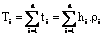is horizontal resistance of multilayered models.

The layer is assumed to be homogeneous and have a thickness H and total vertical conductance S. So, its resistivity r = H/S is equal to its vertical average resistivity.

(7)

Similarly, the vertical average resistivity for multilayered models.

(8)

From eq.(7) and (8), we obtain the average resistivity for multilayered models.

(9)

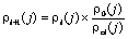
b) Methods for calculating the average resistivity by Dudás fomulas

Using the parameters obtained from the automatic interpretation by Zohdy method, including the resistivity r and layer thickness m, the average resistivities are determined by Dudás formulas.

· The average resistivity r_0hj calculated from the surface down to depth h_j is:

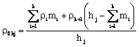(10)

where 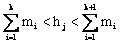, j = 1, 2, …

· The average resistivity r_(hj-1)-hj for depth intervals (from h_j-1 to h_j) is:

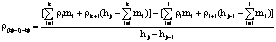where and

II. RESULTS OF APPLICATION

1. Geology and hydrogeology

Almost area of the Hồ Chí Minh City is covered by Neogene-Quaternary sediments. From the surface of the earth, there exist 2 first sediment beds:

- Holocene sediments: unconsolidated ones, including clay, silt and sand, 20-30 m thick.

- Pleistocene sediments: consolidated ones, including sand, gravel, …

and the first two aquifers :

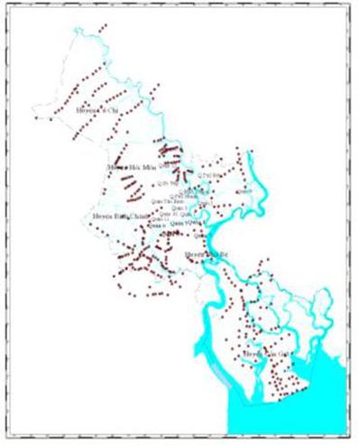
Figure 2. Map of field data points in Hồ Chí Minh city

- Holocene aquifer (qh): distributed in narrow areas of Bình Chánh and Cần Giờ districts, 8 m thick;

- Pleistocene aquifer (qp): distributed all over the City, including the City centre, Tân Bình, 2, 9, Thủ Đức, Hóc Môn and Củ Chi districts.

2. Average resistivity maps

Over 500 field data points in Hồ Chí Minh City have been collected (Fig. 2). From these data the average resistivity maps are built by the both above methods for the sequence lying between 0 and 5 m and 5 and 10 m, respectively. The same results are obtained that are presented in Figs. 3a, b and 4a, b.

The maps show that the average resistivities of Hồ Chí Minh City change in a large range from 2 to hundreds ohm-m, in which Cần Giờ, Bình Chánh, 8, Nhà Bè district areas have low or very low resistivity values, less than 2.0 ohm-m, indicating saline zones. This is an advantage for connecting to ground and designing lightning-conductors, but a disadvantage for protecting the buildings from electrochemical effect.

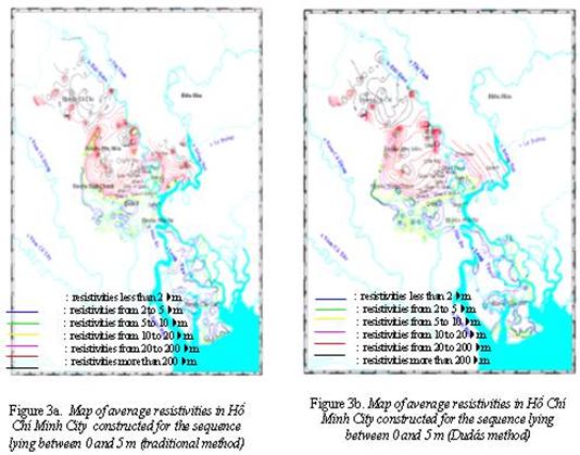
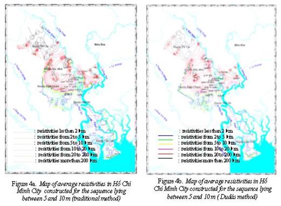
Meanwhile, the Thủ Đức, Hóc Môn, Gò Vấp and Tân Bình districts have high average resistivity values, more than 20 ohm-m, especially the Củ Chi district has very high resistivity values, over 200 ohm-m. Other areas have average resistivity values, from 5 to 20 ohm-m.

III. DISCUSSION

The average resistivity maps for different depths in Hồ Chí Minh City were built from reliable data. The automatic interpretation of sounding curves using Abramova’s filter with 15 filter coefficients does not make a noise when the geological medium is complex. Moreover, this method does not depend subjectively on interpreters. The results obtained by traditional and Dudás formulars are the same, which could be made reference to designing the buildings related to conductivity in Hồ Chí Minh City areas.

REFERENCES

1. Dudas J., 1994. Methodological experience of geoelectric studies of young sediments of the Little Plain. Geoph. Trans., 39 : 2-3. Eotvos Lorand Geoph. Inst. of Hungary.

2. Hoai Thanh D., Ngoc Thu N., Thanh Van N., 2005. Calculating average resistivities of Hồ Chí Minh City by Barnes method. Proc. 4^th Vietnamese Techn. and Sci. Conf. of Geophysics, pp. 537-545. Hà Nội.

3. Khomelevskoi V.K., Shevnin V.A., 1998. Resistivity sounding measurements in geological medium. Lomonosov University, Moscow.

4. Koefoed Otto, 1979. Geosounding principles. 1. Resistivity sounding measure-ments. Delft Univ. of Techn..

5. Ngoc Thanh Le, 1999. Average resistivity map of Mekong river banks. Sub-Institute of Geography, VAST. Hồ Chí Minh City.

6. Loke M.H., Barker R.D., 1994. Improvements to the Zohdy method for the inversion of resistivity sounding and pseudosection data. School of Earth Sci., The Univ. of Birmingham, Edgbaston. Birmingham.

7. Zohdy A.A.R., 1989. A new method for the automatic interpretation of Schlum-berger and Wenner sounding curves. Geophysics, 54 : 245-253.